Forward Kinematics First: You Can't Solve IK Without It
Before solving inverse kinematics, you need forward kinematics (FK) — computing the end-effector's pose from known joint angles. This is done using Denavit-Hartenberg (DH) parameters, a standard way to describe each joint's geometry with four values: link length (a), link twist (α), link offset (d), and joint angle (θ).
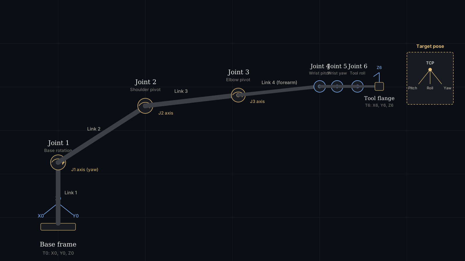
Each joint's transformation is a 4×4 homogeneous matrix. Multiplying all six matrices together gives the full transform from the base to the end-effector.
# Standard DH transformation matrix and forward kinematics chain
import numpy as np

def dh_matrix(theta, d, a, alpha):
    ct, st = np.cos(theta), np.sin(theta)
    ca, sa = np.cos(alpha), np.sin(alpha)
    return np.array([
        [ct, -st * ca,  st * sa, a * ct],
        [st,  ct * ca, -ct * sa, a * st],
        [0,       sa,       ca,      d],
        [0,        0,        0,      1]
    ])

def forward_kinematics(dh_table, joint_angles):
    # dh_table: list of (d, a, alpha, theta_offset) per joint
    # joint_angles: list of 6 variable joint angles (radians)
    T = np.eye(4)
    for (d, a, alpha, offset), theta in zip(dh_table, joint_angles):
        T = T @ dh_matrix(theta + offset, d, a, alpha)
    return T  # 4x4 pose: T[:3,:3] = rotation, T[:3,3] = position
The dh_table values are specific to your robot's geometry — link lengths and joint offsets from its mechanical design. Every solver below builds on this function.
Geometric IK for a Spherical-Wrist Arm (the Fast, Analytical Method)
Most industrial 6-DOF arms — and a large share of hobby arms modeled after them — use a spherical wrist design: the axes of joints 4, 5, and 6 all intersect at one point. This geometric property lets you decouple the problem into two much simpler sub-problems instead of solving six equations simultaneously:
- Position (joints 1-3): Solve where the wrist center needs to be, using triangle geometry.
- Orientation (joints 4-6): Solve the remaining rotation once the wrist center position is fixed.
Step 1 — Find the Wrist Center
The wrist center is offset from the target end-effector position along the tool's approach direction (the Z-axis of the target rotation matrix) by the wrist-to-flange distance, d6:
def wrist_center(target_pos, target_rot, d6):
    approach_vector = target_rot[:, 2]  # Z-axis column of target rotation matrix
    return target_pos - d6 * approach_vector
Step 2 — Solve Joints 1, 2, 3 (Position)
With the wrist center known, joint 1 is a simple base rotation, and joints 2-3 form a triangle with the two link lengths — solved using the law of cosines:
def solve_position(wx, wy, wz, a1, a2, a3, d1, elbow_up=True):
    theta1 = np.arctan2(wy, wx)

    r = np.sqrt(wx**2 + wy**2) - a1
    s = wz - d1
    D = (r**2 + s**2 - a2**2 - a3**2) / (2 * a2 * a3)
    D = np.clip(D, -1.0, 1.0)  # guard against floating-point domain errors

    theta3 = np.arctan2(np.sqrt(1 - D**2), D) if elbow_up else np.arctan2(-np.sqrt(1 - D**2), D)
    theta2 = np.arctan2(s, r) - np.arctan2(a3 * np.sin(theta3), a2 + a3 * np.cos(theta3))

    return theta1, theta2, theta3
Note the elbow_up flag: the ± in front of the square root produces two valid solutions — "elbow up" and "elbow down." Real IK code always has to choose between multiple valid configurations; simply taking the first solution found is a common bug that causes the arm to unexpectedly flip posture between nearby targets.
Step 3 — Solve Joints 4, 5, 6 (Orientation)
Once joints 1-3 are known, compute the rotation matrix they produce (R0_3), then isolate the remaining rotation the wrist must contribute:
def solve_orientation(R0_3, R_target):
    R3_6 = R0_3.T @ R_target  # remaining rotation after removing joints 1-3

    theta5 = np.arctan2(np.sqrt(R3_6[0,2]**2 + R3_6[1,2]**2), R3_6[2,2])
    # wrist-flip case: theta5 ≈ 0 is a singularity, handled separately below
    if abs(np.sin(theta5)) > 1e-6:
        theta4 = np.arctan2(R3_6[1,2], R3_6[0,2])
        theta6 = np.arctan2(R3_6[2,1], -R3_6[2,0])
    else:
        # Wrist singularity: theta4 and theta6 become coupled (infinite solutions)
        # Convention: fix theta4 = 0 and fold all rotation into theta6
        theta4 = 0.0
        theta6 = np.arctan2(-R3_6[0,1], R3_6[0,0])

    return theta4, theta5, theta6
theta5 approaches zero, joint 4 and joint 6 axes align, and the split above between them becomes arbitrary — there are infinitely many (θ4, θ6) pairs that produce the same orientation. Production robot controllers detect proximity to this condition and either warn the operator or slow the motion to avoid the near-infinite joint velocities it can otherwise demand.
Numerical IK: The Jacobian Method (When There's No Clean Geometry)
The geometric method above only works cleanly because of the spherical wrist assumption. For arms without that property — unusual joint configurations, redundant arms, or when you need to respect joint limits and avoid obstacles — the standard approach is iterative: start from a guess, and nudge the joint angles toward the target using the Jacobian matrix (which relates small joint movements to small end-effector movements).
def numerical_jacobian(dh_table, angles, epsilon=1e-6):
    n = len(angles)
    J = np.zeros((6, n))
    T0 = forward_kinematics(dh_table, angles)
    p0, R0 = T0[:3, 3], T0[:3, :3]

    for i in range(n):
        perturbed = angles.copy()
        perturbed[i] += epsilon
        Ti = forward_kinematics(dh_table, perturbed)
        pi, Ri = Ti[:3, 3], Ti[:3, :3]

        J[:3, i] = (pi - p0) / epsilon               # linear velocity part
        dR = Ri @ R0.T
        J[3:, i] = np.array([dR[2,1], dR[0,2], dR[1,0]]) / epsilon  # angular velocity part

    return J

def jacobian_ik(dh_table, target_pos, target_rot, initial_angles,
                 max_iters=200, tol=1e-4, damping=0.01):
    theta = np.array(initial_angles, dtype=float)

    for _ in range(max_iters):
        T = forward_kinematics(dh_table, theta)
        pos_error = target_pos - T[:3, 3]
        rot_error_matrix = target_rot @ T[:3, :3].T
        rot_error = np.array([
            rot_error_matrix[2,1] - rot_error_matrix[1,2],
            rot_error_matrix[0,2] - rot_error_matrix[2,0],
            rot_error_matrix[1,0] - rot_error_matrix[0,1]
        ]) * 0.5
        error = np.concatenate([pos_error, rot_error])

        if np.linalg.norm(error) < tol:
            return theta, True   # converged

        J = numerical_jacobian(dh_table, theta)
        # Damped least-squares (avoids instability near singularities)
        JT = J.T
        delta = JT @ np.linalg.solve(J @ JT + (damping**2) * np.eye(6), error)
        theta += delta

    return theta, False  # did not converge within max_iters
The damping term implements the Damped Least Squares (DLS) method instead of a raw Jacobian pseudo-inverse. Without damping, the solver produces wild, unstable joint jumps when the arm passes near a singularity — the pseudo-inverse of a near-singular Jacobian has enormous values. DLS trades a small amount of accuracy for numerical stability, which is the standard tradeoff used in libraries like Orocos KDL.
C++ Implementation Using Eigen
For real-time control loops running on an industrial PC or embedded Linux board, the same math ported to C++ with the Eigen linear algebra library runs orders of magnitude faster than the Python/NumPy version, since it avoids interpreter overhead entirely:
#include <Eigen/Dense>
#include <cmath>

Eigen::Matrix4d dhMatrix(double theta, double d, double a, double alpha) {
    double ct = std::cos(theta), st = std::sin(theta);
    double ca = std::cos(alpha), sa = std::sin(alpha);

    Eigen::Matrix4d T;
    T << ct, -st*ca,  st*sa, a*ct,
         st,  ct*ca, -ct*sa, a*st,
          0,     sa,     ca,    d,
          0,      0,      0,    1;
    return T;
}

Eigen::Matrix4d forwardKinematics(const std::vector<std::array<double,4>>& dhTable,
                                   const std::vector<double>& jointAngles) {
    Eigen::Matrix4d T = Eigen::Matrix4d::Identity();
    for (size_t i = 0; i < dhTable.size(); ++i) {
        double d = dhTable[i][0], a = dhTable[i][1];
        double alpha = dhTable[i][2], offset = dhTable[i][3];
        T = T * dhMatrix(jointAngles[i] + offset, d, a, alpha);
    }
    return T;
}
The Jacobian-based numerical solver follows the identical structure shown in Python — Eigen's JacobiSVD or ColPivHouseholderQR classes handle the damped least-squares solve shown earlier with a single method call, avoiding a hand-rolled matrix inversion.
Arduino: What's Actually Realistic
Here's the honest answer most tutorials skip: a full 6-DOF geometric IK solve involves multiple atan2, acos, and sqrt calls per solve. An 8-bit Arduino Uno (ATmega328P, no hardware FPU, 16 MHz) can technically compute this, but each trig call costs hundreds of microseconds in software floating point — for a single IK solve this is often fine for slow point-to-point motion, but too slow for continuous real-time trajectory tracking.
Two realistic paths:
- Run IK off-board. Compute joint angles in Python or C++ on a host computer or Raspberry Pi, and stream the six resulting angles to the Arduino over serial as simple servo commands. This is the standard architecture for DIY arms and keeps the microcontroller's job trivial: read serial, write to servos.
- Use a 32-bit board for on-board IK. An ESP32 or Teensy 4.x has a real floating-point unit and runs the same geometric solver shown above comfortably fast enough for smooth motion, with no host PC required.
For a simpler on-board case that an Arduino Uno handles well, here's geometric IK for a 4-DOF arm (base rotation + shoulder + elbow + wrist pitch) — common in low-cost educational kits and light enough for 8-bit hardware:
// 4-DOF geometric IK: base, shoulder, elbow, wrist pitch
// L1 = shoulder-to-elbow length, L2 = elbow-to-wrist length (mm)

bool solveIK4DOF(float x, float y, float z, float L1, float L2,
                  float& baseAngle, float& shoulderAngle, float& elbowAngle) {
    baseAngle = atan2(y, x);

    float r = sqrt(x*x + y*y);
    float D = (r*r + z*z - L1*L1 - L2*L2) / (2 * L1 * L2);

    if (D < -1.0 || D > 1.0) return false;  // target unreachable

    elbowAngle = acos(D);  // elbow-down solution
    shoulderAngle = atan2(z, r) - atan2(L2 * sin(elbowAngle), L1 + L2 * cos(elbowAngle));

    return true;  // true = valid solution found
}

void loop() {
    float baseA, shoulderA, elbowA;
    if (solveIK4DOF(150, 50, 100, 120, 100, baseA, shoulderA, elbowA)) {
        // Convert radians to servo microseconds/degrees and write here
    }
    // else: target out of reach — skip the move, don't send garbage angles
}
D falls outside [-1, 1], the target is geometrically unreachable and acos() will return NaN in software floating point — silently sending that to a servo can cause unpredictable jumps. Reject the command instead of feeding it downstream.
Open-Source Libraries Worth Using Instead of Writing Your Own
Writing your own solver is valuable for learning and for simple arms, but for production use, these maintained open-source projects handle joint limits, singularities, and multiple robot geometries more robustly than a first custom implementation typically will:
Geometric vs. Numerical: When to Use Each
| Property | Geometric (Spherical Wrist) | Numerical (Jacobian/DLS) |
|---|---|---|
| Speed | Very fast — closed-form, fixed number of operations | Slower — iterative, variable number of steps to converge |
| Requires spherical wrist | Yes | No — works for any joint configuration |
| Multiple solutions | Explicit (elbow up/down, wrist flip) — you choose | Converges to whichever solution is nearest the initial guess |
| Behavior near singularities | Can produce large joint jumps if not detected explicitly | Degrades gracefully with damping, but may fail to converge |
| Best suited for | Fixed-geometry industrial/collaborative arms with known DH parameters | Redundant arms, unusual geometries, obstacle-aware motion |
Testing Your IK Solver Before Trusting It on Real Hardware
The single most useful sanity check for any IK implementation is a round-trip test: run forward kinematics on a set of known joint angles to get a target pose, feed that pose into your IK solver, and confirm it returns joint angles that produce the same pose when run back through forward kinematics.
test_angles = [0.3, -0.5, 1.1, 0.0, 0.7, -0.2]
T_target = forward_kinematics(dh_table, test_angles)

solved_angles, converged = jacobian_ik(
    dh_table, T_target[:3,3], T_target[:3,:3], initial_angles=[0]*6
)

T_check = forward_kinematics(dh_table, solved_angles)
position_error = np.linalg.norm(T_target[:3,3] - T_check[:3,3])

assert converged and position_error < 1e-3, "IK solver failed round-trip test"
Run this across a grid of random joint angles spanning your robot's full range of motion, including configurations near singularities, before deploying any solver — geometric or numerical — to real hardware.
"An IK solver that works for one target pose and fails silently near a singularity is more dangerous than one that visibly fails everywhere — test the edges of your workspace, not just the center."— Robotics Engineering, Motion Control Editorial Notes
Sources and Further Reading
- Craig, J. J. — Introduction to Robotics: Mechanics and Control. The standard reference for DH parameter conventions and the geometric spherical-wrist decoupling method used in this article.
- Orocos Kinematics and Dynamics Library (KDL) — reference implementation of damped least-squares IK used throughout the ROS ecosystem.
- MoveIt 2 Documentation — kinematics plugin architecture and solver comparison.
- Eigen — C++ linear algebra library used in the C++ examples above.
- ikpy — open-source Python IK library referenced for practical implementation.
Code samples in this article are illustrative implementations of well-established algorithms, simplified for clarity. Production use should include joint limit clamping, singularity detection, and validation against your specific robot's DH parameters.
What's the difference between forward and inverse kinematics?
Forward kinematics calculates the end-effector's position and orientation from known joint angles — a direct calculation with one unique answer. Inverse kinematics does the opposite: given a target position and orientation, it solves for the joint angles needed to reach it, and for a 6-DOF arm this can have multiple valid solutions or none at all.
Why do most 6-DOF robot arms use a spherical wrist design?
A spherical wrist means the last three joint axes intersect at a single point, letting you split inverse kinematics into a position problem (joints 1-3) and an orientation problem (joints 4-6). Without this decoupling, you generally need slower numerical methods to solve all six joints simultaneously.
Can a low-cost microcontroller like an Arduino Uno run 6-DOF inverse kinematics in real time?
An 8-bit Arduino Uno struggles with the trigonometric calls needed for full 6-DOF geometric IK at high control rates since it lacks a hardware floating-point unit. A 32-bit board like an ESP32 or Teensy handles it comfortably, or you can compute IK on a host PC and stream joint angles to the Arduino over serial.
What is a kinematic singularity and why does it matter for IK code?
A singularity is an arm configuration where the Jacobian matrix loses rank, meaning the arm momentarily loses a degree of freedom — for example, when wrist axes align. Near a singularity, small changes in desired end-effector position can require very large or physically impossible joint velocity changes, which is why production IK code detects and handles these cases explicitly.
Related Reading
- ROS 2 Control Architecture for 6-DOF Robot Arms
- Arduino 6-DOF Robot Arm Tutorial: Wiring, Code & Calibration
- ESP32 as Robot Arm Controller: Performance, WiFi & Bluetooth Integration
- The Complete 6-DOF Robot Arm Guide (2026)
Primary sources and further reading
These references support the general engineering concepts in this guide. Component limits vary by variant and revision; check the governing datasheet.
Links checked: August 5, 2026.