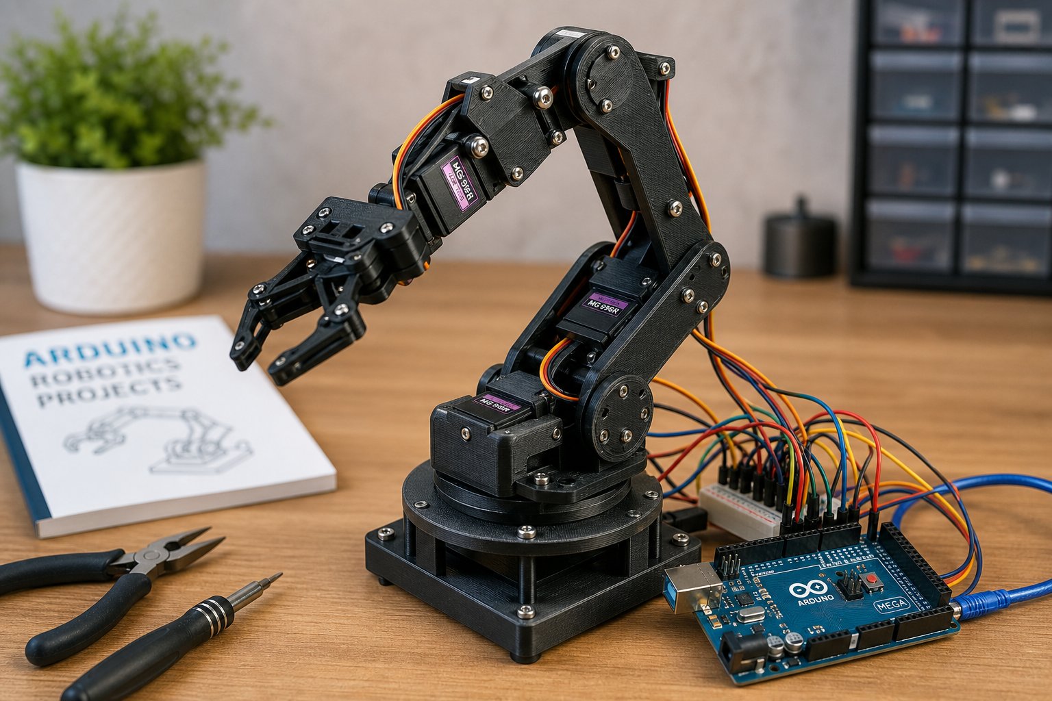
What Inverse Kinematics Actually Solves
Every 6-DOF robot arm has two related but opposite math problems to solve. Forward kinematics (FK) answers: "If I set joints 1 through 6 to these specific angles, where will the gripper end up in 3D space?" This is a straightforward calculation — you always get exactly one answer, computed by chaining together rotation and translation matrices for each joint.
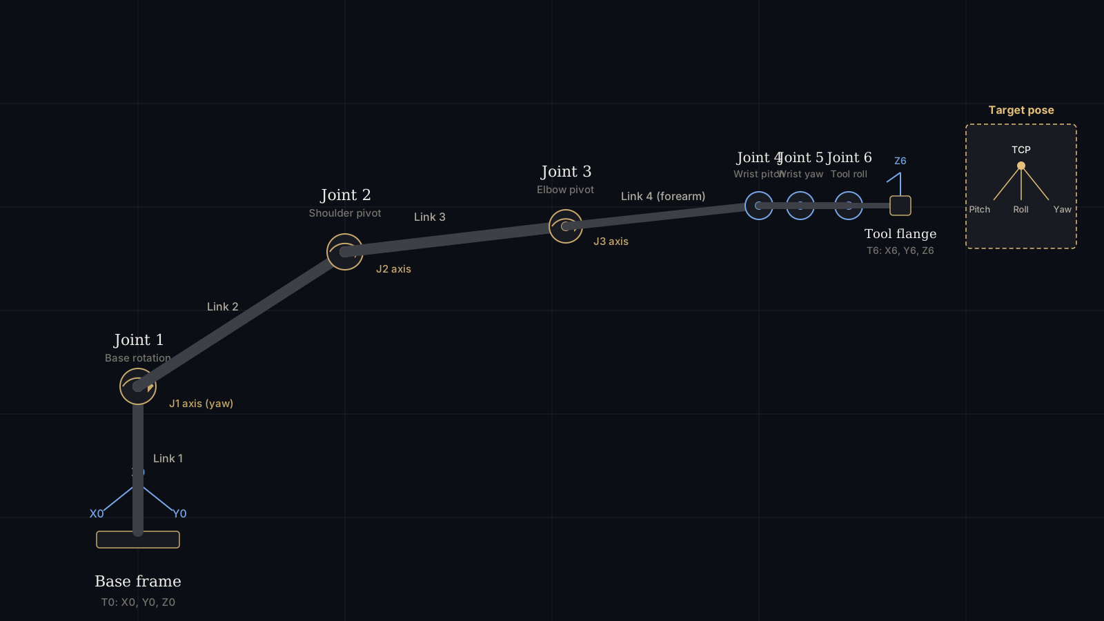
Inverse kinematics (IK) asks the opposite question: "I want the gripper at this exact position and orientation — what should each of the six joint angles be?" This is dramatically harder. Unlike forward kinematics, inverse kinematics can have zero solutions (the point is unreachable), exactly one solution, multiple valid solutions (the same point reached with the elbow up or down), or infinite solutions (in redundant robots with more than 6 joints).
This guide walks through the analytical method used by most industrial 6-DOF arms, works through a complete numerical example with real numbers, and provides functional code you can run in Python, adapt for Arduino, or integrate with ROS 2's MoveIt framework.
The Geometry: Why 6 Joints and Not 5 or 7
A rigid object in 3D space has six degrees of freedom: three for position (X, Y, Z) and three for orientation (roll, pitch, yaw). This is precisely why standard industrial robot arms use six joints — it's the minimum number required to place the end-effector at any reachable position with any desired orientation.
Most 6-DOF industrial arms use a specific joint arrangement called a spherical wrist, where joints 4, 5, and 6 all intersect at a single point. This isn't an arbitrary design choice — it's what makes the analytical (closed-form) solution to inverse kinematics possible. Without this geometric property, solving IK typically requires slower iterative numerical methods.
Denavit-Hartenberg (DH) Parameters: The Foundation
Before solving IK, you need a standardized way to describe your robot's geometry. The Denavit-Hartenberg convention assigns four parameters to each joint, describing how its coordinate frame relates to the previous joint's frame:
| Parameter | Symbol | Description |
|---|---|---|
| Link length | a | Distance between joint axes along the common normal |
| Link twist | α (alpha) | Angle between joint axes, measured about the common normal |
| Link offset | d | Distance along the previous joint's axis to the common normal |
| Joint angle | θ (theta) | Rotation angle about the joint's own axis — this is the variable IK solves for |
Example DH table for a generic 6-DOF arm (values in mm and degrees, representative of a mid-size industrial arm):
| Joint | a (mm) | α (°) | d (mm) | θ (variable) |
|---|---|---|---|---|
| 1 | 0 | -90 | 333 | θ1 |
| 2 | 340 | 0 | 0 | θ2 |
| 3 | 0 | -90 | 0 | θ3 |
| 4 | 0 | 90 | 340 | θ4 |
| 5 | 0 | -90 | 0 | θ5 |
| 6 | 0 | 0 | 80 | θ6 |
The Analytical Solution: Wrist-Position Decoupling
The key trick that makes 6-DOF analytical IK manageable is splitting the problem into two independent 3-DOF problems, made possible by the spherical wrist geometry described above.
Step 1: Solve for Wrist Center Position (Joints 1-3)
First, calculate the position of the wrist center — the point where joints 4, 5, and 6 intersect — by working backward from the desired end-effector pose:
Where d6 is the distance from the wrist center to the tool tip, and R is the desired end-effector rotation matrix. Once you know the wrist center's (X, Y, Z) position, joints 1, 2, and 3 can be solved using standard trigonometry (law of cosines) as if solving a simpler 3-DOF planar arm:
θ3 = atan2(±√(1 − D²), D), where D = (r² + s² − a2² − a3²) / (2·a2·a3)
θ2 = atan2(s, r) − atan2(a3·sin(θ3), a2 + a3·cos(θ3))
The ± in the θ3 equation is exactly why IK often has two valid solutions for position — one with the "elbow up" and one with "elbow down."
Step 2: Solve for Wrist Orientation (Joints 4-6)
With joints 1-3 fixed, calculate the rotation matrix that joints 4-6 need to produce by isolating it: R36 = R03⁻¹ · R06. Then extract the three wrist joint angles from this matrix using the standard ZYZ Euler angle decomposition:
θ4 = atan2(R36[1,2], R36[0,2])
θ6 = atan2(R36[2,1], −R36[2,0])
When θ5 is near zero, joints 4 and 6 become rotationally aligned — this is the wrist singularity mentioned in the FAQ below, and it requires special handling in real controllers to avoid erratic joint motion.
Worked Numerical Example
Let's solve for joints 1-3 using a simplified 2-link planar case with real numbers, using link lengths a2 = 340mm and a3 = 340mm, targeting a wrist center at r = 450mm (horizontal distance), s = 200mm (vertical distance):
D = (450² + 200² − 340² − 340²) / (2 × 340 × 340)
D = (202500 + 40000 − 115600 − 115600) / 231200
D = 11300 / 231200
D = 0.0489

θ3 = atan2(√(1 − 0.0489²), 0.0489)
θ3 = atan2(0.9988, 0.0489)
θ3 ≈ 87.2°  (elbow-up solution)

θ2 = atan2(200, 450) − atan2(340 × sin(87.2°), 340 + 340 × cos(87.2°))
θ2 = 23.96° − atan2(339.6, 356.9)
θ2 = 23.96° − 43.55°
θ2 ≈ −19.6°
This confirms the wrist center is reachable with θ2 ≈ -19.6° and θ3 ≈ 87.2° — you would repeat this with the negative square root for the alternative "elbow-down" solution.
Python Implementation
The following Python function implements the position-solving portion (joints 1-3) described above, using NumPy for matrix operations:
Python — analytical_ik.pyimport numpy as np
def solve_joints_1_to_3(px, py, pz, a2, a3, d1):
"""
Solves the first three joint angles for a 6-DOF arm
given the wrist center position (px, py, pz).
Returns both elbow-up and elbow-down solutions.
"""
theta1 = np.arctan2(py, px)
r = np.sqrt(px**2 + py**2)
s = pz - d1
D = (r**2 + s**2 - a2**2 - a3**2) / (2 * a2 * a3)
D = np.clip(D, -1.0, 1.0) # guard against floating point errors
theta3_up = np.arctan2(np.sqrt(1 - D**2), D)
theta3_down = np.arctan2(-np.sqrt(1 - D**2), D)
def solve_theta2(theta3):
return (np.arctan2(s, r) -
np.arctan2(a3 * np.sin(theta3), a2 + a3 * np.cos(theta3)))
theta2_up = solve_theta2(theta3_up)
theta2_down = solve_theta2(theta3_down)
return {
"elbow_up": (theta1, theta2_up, theta3_up),
"elbow_down": (theta1, theta2_down, theta3_down)
}
# Example usage with the numbers from the worked example above
solution = solve_joints_1_to_3(px=450, py=0, pz=200, a2=340, a3=340, d1=0)
theta1, theta2, theta3 = solution["elbow_up"]
print(f"θ1={np.degrees(theta1):.1f}°, θ2={np.degrees(theta2):.1f}°, θ3={np.degrees(theta3):.1f}°")
# Output: θ1=0.0°, θ2=-19.6°, θ3=87.2°Arduino Implementation Notes
Running full 6-DOF analytical IK on an Arduino Uno (ATmega328P, 16MHz, no floating-point unit) is computationally feasible but requires care, since trigonometric functions are relatively expensive on 8-bit microcontrollers. An Arduino Mega or ESP32 handles this comfortably; a base Arduino Uno benefits from precomputed lookup tables.
Arduino C++ — simplified 3-DOF IK for servo control#include <math.h>
struct JointAngles {
float theta1, theta2, theta3;
};
JointAngles solveIK(float px, float py, float pz, float a2, float a3) {
JointAngles result;
result.theta1 = atan2(py, px);
float r = sqrt(px * px + py * py);
float s = pz;
float D = (r * r + s * s - a2 * a2 - a3 * a3) / (2 * a2 * a3);
D = constrain(D, -1.0, 1.0);
result.theta3 = atan2(sqrt(1 - D * D), D);
result.theta2 = atan2(s, r) -
atan2(a3 * sin(result.theta3), a2 + a3 * cos(result.theta3));
return result;
}
void setup() {
Serial.begin(9600);
JointAngles angles = solveIK(450, 0, 200, 340, 340);
// Convert radians to degrees for servo.write()
int servo1Angle = degrees(angles.theta1) + 90; // offset for servo center
int servo2Angle = degrees(angles.theta2) + 90;
int servo3Angle = degrees(angles.theta3) + 90;
Serial.print("Servo angles: ");
Serial.print(servo1Angle); Serial.print(", ");
Serial.print(servo2Angle); Serial.print(", ");
Serial.println(servo3Angle);
}
void loop() {}ROS 2 and MoveIt: Numerical IK for Complex Cases
While analytical IK is fast and predictable, it only works cleanly for arms with a spherical wrist and doesn't handle additional constraints like obstacle avoidance or joint limit optimization. This is where ROS 2's MoveIt framework becomes valuable — it uses numerical IK solvers (KDL, TRAC-IK, or BioIK) that iteratively converge on a solution rather than computing it in closed form.
ROS 2 — requesting an IK solution via MoveIt Python APIfrom moveit.planning import MoveItPy
from geometry_msgs.msg import PoseStamped
def request_ik_solution(moveit_instance, target_pose: PoseStamped):
arm = moveit_instance.get_planning_component("arm_group")
arm.set_goal_state(pose_stamped_msg=target_pose, pose_link="tool0")
plan_result = arm.plan()
if plan_result:
joint_trajectory = plan_result.trajectory
return joint_trajectory
else:
raise RuntimeError("No IK solution found for target pose")MoveIt's numerical solvers typically take 5-10 milliseconds per query — noticeably slower than the sub-2-millisecond analytical method, but this overhead is usually acceptable for motion planning tasks that aren't running in a tight real-time control loop.
| Method | Typical Solve Time | Best For | Limitation |
|---|---|---|---|
| Analytical (closed-form) | 0.3 - 2 ms | Spherical-wrist arms, real-time control | Requires specific joint geometry |
| KDL (ROS 2 default) | 5 - 15 ms | General-purpose, any joint configuration | Can fail to converge near singularities |
| TRAC-IK | 1 - 8 ms | Faster convergence, redundant arms | Slightly more complex setup |
Common Pitfalls When Implementing IK
- Ignoring the D value out-of-range case: If
|D| > 1in the position equations above, the target point is physically unreachable — always check this before callingarccosorarcsin, or you'll get NaN results that crash downstream code. - Not handling multiple solutions: Real IK problems often have 2-8 valid joint configurations for a single target pose. Always implement a solution-selection strategy (closest to current joint angles is the most common approach) rather than arbitrarily picking one.
- Forgetting joint limits: A mathematically valid IK solution may require a joint angle outside your servo or motor's physical range. Always validate solutions against actual hardware limits before commanding motion.
- Assuming a spherical wrist without verifying it: If your robot's joint 4, 5, and 6 axes don't actually intersect at one point (common in some low-cost hobby arm kits), the analytical decoupling method described here will produce incorrect results — verify your specific arm's geometry first.
"The spherical wrist isn't just a mechanical convenience — it's the geometric property that turns an otherwise intractable six-equation system into two solvable three-equation problems."— Robotics Engineering, Robotics Fundamentals Series 2026
Related Resources
Continue building your robot arm programming knowledge with these related guides on hardware, control, and vision integration.
- Robot Arm Payload Calculator: How to Size a 6-DOF Arm for Your Load
- Integrating Vision Systems with 6-DOF Robot Arms: Cameras, AI & Grasping
- 6-Axis Robot Arm Maintenance Schedule: Preventive Care for Maximum Uptime
- ESP32 as Robot Arm Controller: Performance, WiFi & Bluetooth Integration
- The Complete 6-DOF Robot Arm Guide (2026)
Sources and References
The mathematical framework and conventions described in this guide follow standard robotics textbook derivations and official documentation from the ROS 2 ecosystem. For deeper theoretical background, consult the following primary references:
- Craig, J.J. — Introduction to Robotics: Mechanics and Control, standard reference for Denavit-Hartenberg convention and analytical IK derivation.
- ROS 2 / MoveIt Documentation — Official kinematics plugin documentation (KDL, TRAC-IK).
- ISO 9787:2013 — Manipulating industrial robots, coordinate systems and motion nomenclature.
- IFR (International Federation of Robotics) — Industrial robot kinematic architecture classification standards.
Frequently Asked Questions
What is the difference between forward and inverse kinematics?
Forward kinematics calculates the end-effector's position and orientation given known joint angles — it always has exactly one solution. Inverse kinematics does the opposite: given a desired end-effector pose, it calculates the required joint angles, and can have zero, one, multiple, or infinite solutions depending on the target and robot geometry.
Why do 6-DOF robot arms use a spherical wrist for inverse kinematics?
A spherical wrist means joints 4, 5, and 6 intersect at a single point, allowing the IK problem to be decoupled into two simpler 3-DOF problems (position and orientation) instead of solving all six equations simultaneously. This is the basis of the fast analytical IK solution used by most industrial controllers.
What is a kinematic singularity?
A kinematic singularity occurs when the robot's Jacobian matrix loses rank, causing the arm to lose a degree of freedom in Cartesian space at that configuration. Near a singularity, small position changes require very large joint velocities. Common examples are wrist singularities and fully-extended elbow singularities.
Should I use analytical or numerical inverse kinematics?
Analytical IK is faster (under 2ms) and ideal for real-time control of spherical-wrist arms. Numerical IK (via ROS 2 MoveIt's KDL or TRAC-IK) is slower but handles arms without a spherical wrist, redundant 7+ DOF arms, and additional constraints like obstacle avoidance.
Primary sources and further reading
These references support the general engineering concepts in this guide. Ratings and limits shown must be confirmed against documentation for your exact configuration.
Links checked: August 5, 2026.